
My Model
This model classifies images from the Brain Tumor dataset with Grad-CAM, you can try out the model on my profile.
Brain Tumor Classification Using InceptionV3 and Grad-CAM
A complete deep learning pipeline for brain tumor classification using MRI scans. This project demonstrates:
- End-to-end data preprocessing
- Augmentation & dataset balancing
- Efficient tf.data pipelines
- Transfer learning with InceptionV3
- Deep model evaluation
- Grad-CAM interpretability
- LaTeX mathematical explanations
1. Dataset Exploration & Inspection
We begin by recursively scanning all MRI images and creating a structured DataFrame:
from pathlib import Path
import pandas as pd

image_extensions = {'.jpg', '.jpeg', '.png'}
paths = [
    (path.parts[-2], path.name, str(path))
    for path in Path("/content/my_data").rglob('*.*')
    if path.suffix.lower() in image_extensions
]

df = pd.DataFrame(paths, columns=['class', 'image', 'full_path'])
df = df.sort_values('class').reset_index(drop=True)
df.head()
Count images per class:
class_count = df['class'].value_counts()
print(class_count)
Visualizations
import matplotlib.pyplot as plt

plt.figure(figsize=(32,16))
class_count.plot(kind='bar', edgecolor='black')
plt.title('Number of Images per Class')
plt.show()
Insights
- Classes are imbalanced
- Images have variable resolution
- Some outliers require cleaning
2. Data Cleaning & Quality Checks
Duplicate removal using MD5 hashes
import hashlib

def get_hash(file_path):
    with open(file_path, 'rb') as f:
        return hashlib.md5(f.read()).hexdigest()

df['file_hash'] = df['full_path'].apply(get_hash)
df_unique = df.drop_duplicates(subset='file_hash', keep='first')
Additional checks
- Corrupted image detection
- Resolution anomalies
- Brightness/contrast outliers
Cleaning ensures a robust dataset with minimal noise.
3. Data Augmentation & Class Balancing
Target ~2,000 images per class using heavy augmentation:
from tensorflow.keras.preprocessing.image import ImageDataGenerator

datagen = ImageDataGenerator(
    rotation_range=20,
    width_shift_range=0.1,
    height_shift_range=0.1,
    shear_range=0.1,
    zoom_range=0.1,
    horizontal_flip=True,
    fill_mode='nearest'
)
Used for minority class upsampling and preventing overfitting.
4. Image Preprocessing Pipeline
import tensorflow as tf

def preprocess_image(path, target_size=(512, 512), augment=True):
    img = tf.io.read_file(path)
    img = tf.image.decode_image(img, channels=3)
    img = tf.image.resize(img, target_size)
    img = tf.cast(img, tf.float32) / 255.0

    if augment:
        img = tf.image.random_flip_left_right(img)
        img = tf.image.random_flip_up_down(img)
        img = tf.image.random_brightness(img, max_delta=0.1)
        img = tf.image.random_contrast(img, 0.9, 1.1)

    return tf.clip_by_value(img, 0.0, 1.0)
- Train set: augmentation enabled
- Validation/Test sets: kept clean
5. Dataset Preparation with tf.data
AUTOTUNE = tf.data.AUTOTUNE
batch_size = 32

train_ds = tf.data.Dataset.from_tensor_slices((train_paths, train_labels))
train_ds = train_ds.shuffle(len(train_paths))
train_ds = train_ds.map(
    lambda x, y: (preprocess_image(x, augment=True), y),
    num_parallel_calls=AUTOTUNE
)
train_ds = train_ds.batch(batch_size).prefetch(AUTOTUNE)
Benefits:
- Parallel loading
- Smart prefetching
- GPU utilization maximized
6. Model Architecture: InceptionV3
Transfer learning from ImageNet:
from tensorflow.keras.applications.inception_v3 import InceptionV3
from tensorflow.keras.layers import GlobalAveragePooling2D, Dense, Dropout
from tensorflow.keras.models import Model

inception = InceptionV3(input_shape=input_shape, weights='imagenet', include_top=False)

for layer in inception.layers:
    layer.trainable = False

x = GlobalAveragePooling2D()(inception.output)
x = Dense(512, activation='relu')(x)
x = Dropout(0.5)(x)
prediction = Dense(len(le.classes_), activation='softmax')(x)

model = Model(inputs=inception.input, outputs=prediction)
Why InceptionV3?
- Factorized convolutions
- Multi-scale feature extraction
- Lightweight and fast
- Strong performance in medical imaging
7. Training & Callbacks
from tensorflow.keras.callbacks import EarlyStopping, ModelCheckpoint, ReduceLROnPlateau

model.compile(
    loss='sparse_categorical_crossentropy',
    optimizer='adam',
    metrics=['accuracy']
)

callbacks = [
    EarlyStopping(monitor='val_loss', patience=40, restore_best_weights=True),
    ModelCheckpoint("best_model.h5", save_best_only=True, monitor='val_loss'),
    ReduceLROnPlateau(monitor='val_loss', factor=0.5, patience=10, min_lr=1e-5)
]
Training:
history = model.fit(train_ds, validation_data=val_ds, epochs=50, callbacks=callbacks)
8. Training Curves
import matplotlib.pyplot as plt

plt.plot(history.history['accuracy'], label='Train Accuracy')
plt.plot(history.history['val_accuracy'], label='Val Accuracy')
plt.title('Training vs Validation Accuracy')
plt.legend()
plt.show()
- Curves indicate smooth convergence
- Small train/val gap → limited overfitting
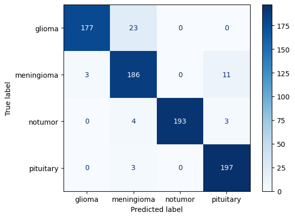
9. Performance Metrics
Confusion Matrix
from sklearn.metrics import confusion_matrix, ConfusionMatrixDisplay

cm = confusion_matrix(y_true, y_pred)
ConfusionMatrixDisplay(cm, display_labels=le.classes_).plot(cmap='Blues')
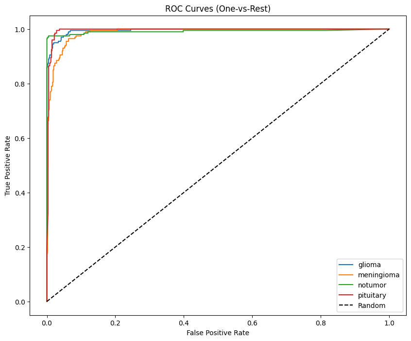
Multi-class AUC (One-vs-Rest)
Macro AUC formula:
from sklearn.preprocessing import label_binarize
from sklearn.metrics import roc_curve, auc

y_true_bin = label_binarize(y_true, classes=np.arange(len(le.classes_)))
10. Grad-CAM: Interpretability
Grad-CAM highlights regions the model uses for classification.
Grad-CAM heatmap:
Where:
Python implementation:
def gradcam(model, img, cls=None):
    # last conv
    lc = next(l for l in reversed(model.layers) if "conv" in l.name.lower())
    gm = tf.keras.Model(model.input, [lc.output, model.output])

    with tf.GradientTape() as t:
        conv, pred = gm(img[None])
        cls = tf.argmax(pred[0]) if cls is None else cls
        loss = pred[:, cls]

    g = t.gradient(loss, conv)
    w = tf.reduce_mean(g, axis=(0,1,2))
    cam = tf.reduce_sum(w * conv[0], -1)

    cam = tf.nn.relu(cam)
    cam /= tf.reduce_max(cam) + 1e-8
    return cam.numpy()
Visualization example:
plt.figure(figsize=(20,10))
for i, img in enumerate(sample_images):
    overlay, info = VizGradCAM(model, img)
    plt.subplot(2, 5, i+1)
    plt.imshow(overlay)
    plt.axis("off")
    plt.title(f"True Label: {le.classes_[sample_labels[i]]}")
plt.show()
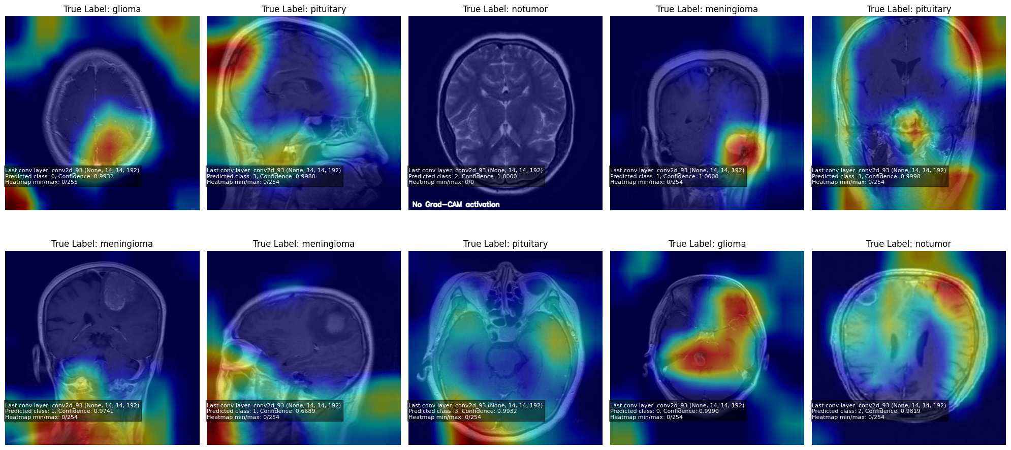
Note: When the model is highly confident in a prediction, the Grad-CAM gradients become near-zero, producing little to no heatmap activation.
11. Technical LaTeX Notes
Sparse Categorical Crossentropy
Global Average Pooling
12. Model Saving
model.save("InceptionV3_Brain_Tumor_MRI.h5")
13. Results
Note: Click the image below to view the video showcasing the project’s results.

Key Takeaways
- Strong data cleaning = reliable model
- Heavy augmentation reduces bias
- InceptionV3 provides excellent feature extraction
- Evaluation metrics reveal clinical reliability
- Grad-CAM adds essential interpretability