
Probabilistic Hyper-Graphs using Multiple Randomly Masked Autoencoders for Semi-supervised Multi-modal Multi-task Learning
Paper
•
2510.10068
•
Published
•
1
The dataset viewer is not available because its heuristics could not detect any supported data files. You can try uploading some data files, or configuring the data files location manually.
Visit the official website for more information: link. This dataset was introduced in our ICCV 2023 workshop paper: link. For citing, see at the end of the page.
![]()
Note: An fully-automated extended variant of this dataset (generating new modalities as inputs) is available at this repository: link.
git lfs install # Make sure you have git-lfs installed (https://git-lfs.com)
git clone https://huggingface.co/datasets/Meehai/dronescapes
Note: the dataset has about 200GB, so it may take a while to clone it.
This is an optional step, but for some use cases, it may be better to use world normals instead of camera normals, which
are provided by default in normals_sfm_manual202204. To convert, we provide camera rotation matrices in
raw_data/camera_matrics.tar.gz for all 8 scenes that also have SfM.
In order to convert, use this function (for each npz file):
def convert_camera_to_world(normals: np.ndarray, rotation_matrix: np.ndarray) -> np.ndarray:
  normals = (normals.copy() - 0.5) * 2 # [-1:1] -> [0:1]
  camera_normals = camera_normals @ np.linalg.inv(rotation_matrix)
  camera_normals = (camera_normals / 2) + 0.5 # [0:1] => [-1:1]
  return np.clip(camera_normals, 0.0, 1.0)
The GPS location (lat/long/height) is in the raw_data/raw_camera_info.tar.gz. Each file over there is an archive over the
original videos, so the train/val/test splits files from raw_data/txt_files must be used to map to proper indices. Each
archive contains a bunch of raw data, however the key lat_long_height should provide the GPS location.
Note: there is no GPS for the norway scene, the log seems to have been lost.
As per the split from the paper:
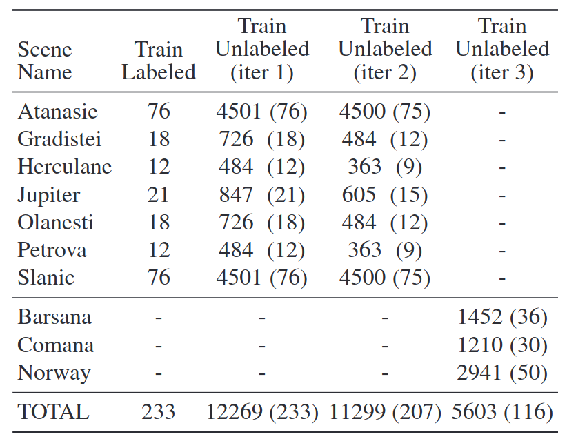
The data is in the data* directory with 1 sub-directory for each split above (and a few more variants).
The simplest way to explore the data is to use the provided notebook. Upon running it, you should get a collage with all the default tasks, like this:

For a CLI-only method, you can use the provided reader as well:
python scripts/dronescapes_viewer.py data/test_set_annotated_only/ # or any of the 8 directories in data/
[MultiTaskDataset]
 - Path: '/export/home/proiecte/aux/mihai_cristian.pirvu/datasets/dronescapes/data/test_set_annotated_only'
 - Tasks (11): [DepthRepresentation(depth_dpt), DepthRepresentation(depth_sfm_manual202204), DepthRepresentation(depth_ufo), ColorRepresentation(edges_dexined), EdgesRepresentation(edges_gb), NpzRepresentation(normals_sfm_manual202204), OpticalFlowRepresentation(opticalflow_rife), ColorRepresentation(rgb), SemanticRepresentation(semantic_mask2former_swin_mapillary_converted), SemanticRepresentation(semantic_segprop8), ColorRepresentation(softseg_gb)]
 - Length: 116
 - Handle missing data mode: 'fill_none'
== Shapes ==
{'depth_dpt': torch.Size([540, 960]),
 'depth_sfm_manual202204': torch.Size([540, 960]),
 'depth_ufo': torch.Size([540, 960, 1]),
 'edges_dexined': torch.Size([540, 960]),
 'edges_gb': torch.Size([540, 960, 1]),
 'normals_sfm_manual202204': torch.Size([540, 960, 3]),
 'opticalflow_rife': torch.Size([540, 960, 2]),
 'rgb': torch.Size([540, 960, 3]),
 'semantic_mask2former_swin_mapillary_converted': torch.Size([540, 960, 8]),
 'semantic_segprop8': torch.Size([540, 960, 8]),
 'softseg_gb': torch.Size([540, 960, 3])}
== Random loaded item ==
{'depth_dpt': tensor[540, 960] n=518400 (2.0Mb) x∈[0.043, 1.000] μ=0.341 σ=0.418,
 'depth_sfm_manual202204': None,
 'depth_ufo': tensor[540, 960, 1] n=518400 (2.0Mb) x∈[0.115, 0.588] μ=0.297 σ=0.138,
 'edges_dexined': tensor[540, 960] n=518400 (2.0Mb) x∈[0.000, 0.004] μ=0.003 σ=0.001,
 'edges_gb': tensor[540, 960, 1] n=518400 (2.0Mb) x∈[0., 1.000] μ=0.063 σ=0.100,
 'normals_sfm_manual202204': None,
 'opticalflow_rife': tensor[540, 960, 2] n=1036800 (4.0Mb) x∈[-0.004, 0.005] μ=0.000 σ=0.000,
 'rgb': tensor[540, 960, 3] n=1555200 (5.9Mb) x∈[0., 1.000] μ=0.392 σ=0.238,
 'semantic_mask2former_swin_mapillary_converted': tensor[540, 960, 8] n=4147200 (16Mb) x∈[0., 1.000] μ=0.125 σ=0.331,
 'semantic_segprop8': tensor[540, 960, 8] n=4147200 (16Mb) x∈[0., 1.000] μ=0.125 σ=0.331,
 'softseg_gb': tensor[540, 960, 3] n=1555200 (5.9Mb) x∈[0., 0.004] μ=0.002 σ=0.001}
== Random loaded batch ==
{'depth_dpt': tensor[5, 540, 960] n=2592000 (9.9Mb) x∈[0.043, 1.000] μ=0.340 σ=0.417,
 'depth_sfm_manual202204': tensor[5, 540, 960] n=2592000 (9.9Mb) NaN!,
 'depth_ufo': tensor[5, 540, 960, 1] n=2592000 (9.9Mb) x∈[0.115, 0.588] μ=0.296 σ=0.137,
 'edges_dexined': tensor[5, 540, 960] n=2592000 (9.9Mb) x∈[0.000, 0.004] μ=0.003 σ=0.001,
 'edges_gb': tensor[5, 540, 960, 1] n=2592000 (9.9Mb) x∈[0., 1.000] μ=0.063 σ=0.102,
 'normals_sfm_manual202204': tensor[5, 540, 960, 3] n=7776000 (30Mb) NaN!,
 'opticalflow_rife': tensor[5, 540, 960, 2] n=5184000 (20Mb) x∈[-0.004, 0.006] μ=0.000 σ=0.000,
 'rgb': tensor[5, 540, 960, 3] n=7776000 (30Mb) x∈[0., 1.000] μ=0.393 σ=0.238,
 'semantic_mask2former_swin_mapillary_converted': tensor[5, 540, 960, 8] n=20736000 (79Mb) x∈[0., 1.000] μ=0.125 σ=0.331,
 'semantic_segprop8': tensor[5, 540, 960, 8] n=20736000 (79Mb) x∈[0., 1.000] μ=0.125 σ=0.331,
 'softseg_gb': tensor[5, 540, 960, 3] n=7776000 (30Mb) x∈[0., 0.004] μ=0.002 σ=0.001}
== Random loaded batch using torch DataLoader ==
{'depth_dpt': tensor[5, 540, 960] n=2592000 (9.9Mb) x∈[0.025, 1.000] μ=0.216 σ=0.343,
 'depth_sfm_manual202204': tensor[5, 540, 960] n=2592000 (9.9Mb) x∈[0., 1.000] μ=0.562 σ=0.335 NaN!,
 'depth_ufo': tensor[5, 540, 960, 1] n=2592000 (9.9Mb) x∈[0.100, 0.580] μ=0.290 σ=0.128,
 'edges_dexined': tensor[5, 540, 960] n=2592000 (9.9Mb) x∈[0.000, 0.004] μ=0.003 σ=0.001,
 'edges_gb': tensor[5, 540, 960, 1] n=2592000 (9.9Mb) x∈[0., 1.000] μ=0.079 σ=0.116,
 'normals_sfm_manual202204': tensor[5, 540, 960, 3] n=7776000 (30Mb) x∈[0.000, 1.000] μ=0.552 σ=0.253 NaN!,
 'opticalflow_rife': tensor[5, 540, 960, 2] n=5184000 (20Mb) x∈[-0.013, 0.016] μ=0.000 σ=0.004,
 'rgb': tensor[5, 540, 960, 3] n=7776000 (30Mb) x∈[0., 1.000] μ=0.338 σ=0.237,
 'semantic_mask2former_swin_mapillary_converted': tensor[5, 540, 960, 8] n=20736000 (79Mb) x∈[0., 1.000] μ=0.125 σ=0.331,
 'semantic_segprop8': tensor[5, 540, 960, 8] n=20736000 (79Mb) x∈[0., 1.000] μ=0.125 σ=0.331,
 'softseg_gb': tensor[5, 540, 960, 3] n=7776000 (30Mb) x∈[0., 0.004] μ=0.002 σ=0.001}
We evaluate in the paper on the 3 test scenes (unsees at train) as well as the semi-supervised scenes (seen, but
different split) against the human annotated frames. The general evaluation script is in
scripts/evaluate_semantic_segmentation.py.
General usage is:
python scripts/evaluate_semantic_segmentation.py y_dir gt_dir -o results.csv --classes C1 C2 .. Cn
[--class_weights W1 W2 ... Wn] [--scenes s1 s2 ... sm]
y_dir and gt_dir Two directories of .npz files in the same format as the datasetclasses A list of classes in the order that they appear in the predictions and gt filesclass_weights (optional, but used in paper) How much to weigh each class. In the paper we compute these weights as
the number of pixels in all the dataset (train/val/semisup/test) for each of the 8 classes resulting in the numbers
below.scenes if the y_dir and gt_dir contains multiple scenes that you want to evaluate separately, the script allows
you to pass the prefix of all the scenes. For example, in data/test_set_annotated_only/semantic_segprop8/ there are
actually 3 scenes in the npz files and in the paper, we evaluate each scene independently. Even though the script
outputs one csv file with predictions for each npz file, the scenes are used for proper aggregation at scene level.python scripts/evaluate_semantic_segmentation.py \
data/test_set_annotated_only/semantic_mask2former_swin_mapillary_converted/ \ # Mask2Former example, use yours here!
data/test_set_annotated_only/semantic_segprop8/ \
-o results.csv \
--classes land forest residential road little-objects water sky hill \
--class_weights 0.28172092 0.30589653 0.13341699 0.05937348 0.00474491 0.05987466 0.08660721 0.06836531 \
--scenes barsana_DJI_0500_0501_combined_sliced_2700_14700 comana_DJI_0881_full norway_210821_DJI_0015_full
Should output:
scene                                             iou      f1
barsana_DJI_0500_0501_combined_sliced_2700_14700  63.371  75.338
comana_DJI_0881_full                              60.559  73.779
norway_210821_DJI_0015_full                       37.986  45.939
mean                                              53.972  65.019
Not providing --scenes will make an average across all 3 scenes (not average after each metric individually):
          iou      f1
scene
all    60.456  73.261
| Model | #paramters | Score (↑) | Barsana (scene 1) | Comana (scene 2) | Norway (scene 3) |
|---|---|---|---|---|---|
| PHG-MAE-Distil{^2} | 4.4M | 56.27 | 66.34 | 61.11 | 37.69 |
| PHG-MAE | 4.4M | 55.32 | 63.80 | 63.18 | 38.98 |
| Mask2Former | 216M | 53.97 | 63.37 | 60.55 | 37.98 |
| NHG(LR) | 32M | 40.76 | 46.51 | 45.59 | 30.17 |
| NHG-Distil | 4.4M | 40.31 | n/a | n/a | n/a |
| CShift{^1} | n/a | 39.67 | 46.27 | 43.67 | 29.09 |
| NGC{^1} | 32M | 35.32 | 44.34 | 38.99 | 22.63 |
| SafeUAV{^1} | 1.1M | 32.79 | n/a | n/a | n/a |
| Model | #paramters | Score (↑) | Barsana (scene 1) | Comana (scene 2) | Norway (scene 3) |
|---|---|---|---|---|---|
| PHG-MAE | 4.4M | 66.09 | 75.98 | 76.12 | 46.18 |
| PHG-MAE-Distil^{2} | 4.4M | 65.60 | 77.21 | 74.47 | 45.13 |
| Mask2Former | 216M | 65.01 | 75.33 | 73.77 | 45.93 |
TODO: provide a simplified (non-weighted) metric which can be used on the entire dataset at once :)
Score is L1 error in meters.
| Model | #paramters | Score (↓) |
|---|---|---|
| PHG-MAE | 4.4M | 16.13 |
| NHG-Distil | 4.4M | 16.64 |
| SafeUAV | 4.4M | 21.66 |
Score is L1 score (in angles) * 100.
| Model | #paramters | Score (↓) |
|---|---|---|
| NHG-Distil | 4.4M | 11.71 |
| PHG-MAE | 4.4M | 12.35 |
| SafeUAV | 4.4M | 12.40 |
One model, three tasks at once. For semantic segmentation, we use Weighted Mean IoU. For the others, the same metric as above.
TODO: combine the three metrics into a single unweighted number. (semantic is [0:100], depth is [0:300] ? and normals is [0:180] or [0:360]).
| Model | #paramters | Semantic Segmentation (↑) | Depth Estimation (↓) | Camera Normals Estimaton (↓) |
|---|---|---|---|---|
| PHG-MAE | 4.4M | 49.74 | 21.60 | 12.80 |
For the real time models, the authors need to provide a self-contained Google Colab notebook. The models must run at >=5FPS on a T4 GPU (free Google Colab instance) for the Dronescapes-Test (or similar) images at 960x540 resolution. We provide an example for the PHG-MAE-Distil 430k parameters model: link.
Notes:
To cite this work, use this:
@InProceedings{Marcu_2023_ICCV,
    author    = {Marcu, Alina and Pirvu, Mihai and Costea, Dragos and Haller, Emanuela and Slusanschi, Emil and Belbachir, Ahmed Nabil and Sukthankar, Rahul and Leordeanu, Marius},
    title     = {Self-Supervised Hypergraphs for Learning Multiple World Interpretations},
    booktitle = {Proceedings of the IEEE/CVF International Conference on Computer Vision (ICCV) Workshops},
    month     = {October},
    year      = {2023},
    pages     = {983-992}
}
and
@misc{mihaicristian2025probabilistichypergraphsusingmultiple,
      title={Probabilistic Hyper-Graphs using Multiple Randomly Masked Autoencoders for Semi-supervised Multi-modal Multi-task Learning},
      author={Pîrvu Mihai-Cristian and Leordeanu Marius},
      year={2025},
      eprint={2510.10068},
      archivePrefix={arXiv},
      primaryClass={cs.CV},
      url={https://arxiv.org/abs/2510.10068},
}
Totally Free + Zero Barriers + No Login Required